
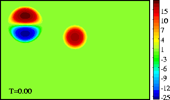
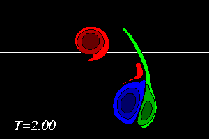
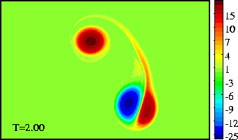
The domain shown is x=[-3.0:+3.0], y=[-2.5:+1.5].
The extrema of voriticity are +/- 29.5 for the dipole
and +23.6 for the monopole.
|
Much to my regret the profider that hosted my webpages for more than 25 years has announced that after 1 July 2026 they end the hosting service. Therefore all my web pages have been moved to another provider, which means the base URL changes from https://josvg.home.xs4all.nl/ to http://www.josvg.dds.nl/. The current page can now be found here. |
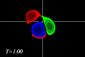
A Lamb dipole with radius 0.75 and
velocity of +2 (i.e. moving to the right) is placed to the
left of a positive Bessel monopole
with radius 0.50 at the origin.
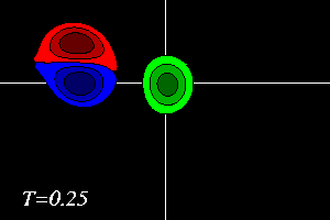
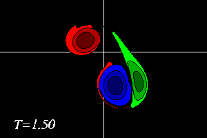
In the main run of this example the dipole is along the x-axis, making the encounter head-on, and the monpole has a circulation of +4, which means that the monopole is weaker than each dipole half.
In this example:
The monopole rotates counter-clockwise, like the top half of the dipole. The result of the rotation is that the dipole is pushed down, to negative y-values, while it moves towards the monopole, like in the run with an offset and a weaker monopole. Since the monopole (green) is in this example stronger, the deformation of the positive dipole half (red) is larger. This can be seen clearest in the tracer plots:
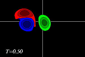
The latter two form a dipolar structure, as in the run with an offset and a weaker monopole, but since the monopole is now nearly as strong as the dipole half, this newly formed dipolar structure moves away from, leaving the original positive dipole half (red) behind as a monopole (though the monopole is still "connected" through a thin vortex band with the dipole, as the red filled counter around the blue dipole half show):
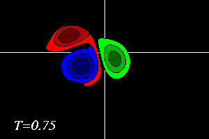

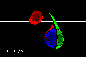
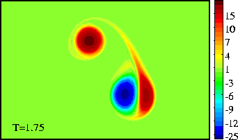
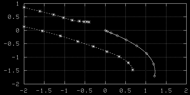
At initialisation, a single tracer particle was placed at the extrema of
vorticity of both vortices. The next graph shows their trajectories:
See the main run of this example, with a weaker monopole and a head-on encounter.
The evolution of the vorticity distribution is computed with a Finite Difference Method which solves the two-dimensional vorticity (Navier-Stokes) equation. Time and distances are given in dimensionless units.
===> Some details on the computation presented on this page for those who are interested.
<=== Numerical simulations of 2D vortex evolution with a Finite Difference Method.
 Jos van Geffen --
Home |
Site Map |
Contact Me
Jos van Geffen --
Home |
Site Map |
Contact Me